In this section I will write a simple and fully working code for Discrete Fourier Transform using Cooley Turkey Method using vector in C++. The application of d-FFT is huge – from communication (Data : Amplitude VS Time) to Michelson Interferometer (Data : Amplitude VS Distance).
Here, I tried to take care all of the problems faced by a new user, as I faced earlier, who is desperately trying to find a working FFT Code and instead of finding some utterly complicated algorithms with ‘*’s and ‘nn’s which does not run on every machine.
Key features of this code are as follows.
- The data in a vector is stored dynamically. So, use of vector eliminates the possibility of ‘Core Dump‘ error which occurs for large size of array.
- In this code, I have taken care of the ‘Zero Filling‘ or ‘Padding‘ of the input Data. This is done to increase the length of the data to a defined length without affecting the quality. To know why it is necessary, you have to read the theory part.
- The above ‘Zero-Filling’ is done in such a way that you can run a non-uniformly spaced data using this code. In d-FFT, you need to feed a data in which all the samples are recored after same interval of unit (i.e. time, distance, etc). But if the data is not in uniformly recorded, this code will take care of that without causing almost no harm to the result. That is why this code is called Pseudo non-Uniform Discrete Fourier Transform.
Mandatory Theory Part
You can jump to the code part if you know this part already. But I will insist you to read a little bit of this theory part in case you need to defend your code to other fellow. It would not be nice if the answer is ‘I got the code from a page called FakePhysicist and do not understand it properly‘. I will try to keep it as simple as possible (as I faced the same difficulties earlier).
First, we will discuss about the d-FFT of uniform data and then will discuss about the ‘Padding’ or ‘Zero-filling’ or ‘Non-uniform to Uniform Conversion’.
The discrete Fourier transform (DFT) of a data x_N is defined by the formula:
X_{k} = \sum_{n=0}^{N-1} x_{n}e^{-\frac{2\pi i}{N}nk}
where k is an integer ranging from 0 to N-1.
As you can see, this is a huge summation of some big-big complex numbers. So, the next thing we do is to break this summation into small-small pieces. And this is the main concept of Cooley Turkey FFT Algorithm.
Now, we can write X_{k} in this way,
\begin{aligned} X_{k} & = \sum_{m=0}^{\frac{N}{2}-1} x_{2m} e^{-\frac{2\pi i}{N}\left(2m\right)k} + \sum_{m=0}^{\frac{N}{2}-1} x_{2m+1} e^{-\frac{2\pi i}{N}\left(2m+1\right)k}\\ & = \underbrace{\left(\sum_{m=0}^{\frac{N}{2}-1} x_{2m} e^{-\frac{2\pi i}{N}\left(2m\right)k}\right)}_\text{Even} + e^{-\frac{2\pi i}{N}k} \underbrace{ \left( \sum_{m=0}^{\frac{N}{2}-1} x_{2m+1} e^{-\frac{2\pi i}{N}\left(2m\right)k}\right)}_\text{Odd}\\ & = E_{k} + e^{-\frac{2\pi i}{N}k} O_{k} \end{aligned}
So, the DFT can be expressed in two terms – Even (E_{k}) and Odd (O_{k}) parts, each consisting of \frac{N}{2} samples of data.
It also can be seen that
\begin{aligned}E_{k+\frac{N}{2}} &= \sum_{m=0}^{\frac{N}{2}-1} x_{2m} e^{-\frac{2\pi i}{N}\left(2m\right)\left(k+\frac{N}{2}\right)}\\ & = \sum_{m=0}^{\frac{N}{2}-1} x_{2m} e^{-\frac{2\pi i}{N}\left(2m\right)k} e^{-2\pi i m} = E_{k}\\ \text{and, } O_{k+\frac{N}{2}} &= O_{k}\end{aligned}.So, we can rewrite the second half of X_{k} as
X_{k}=\left\{\begin{array}{ll}E_{k}+e^{-\frac{2\pi i}{N}k} O_{k} & \text{ for } 0 \leq k< \frac{N}{2} \\ E_{k-\frac{N}{2}}+e^{-\frac{2\pi i}{N}k} O_{k-\frac{N}{2}} & \text{ for } \frac{N}{2} \leq k < N \end{array} \right.
By replacing k with k+\frac{N}{2} in the second half, we can find
\begin{aligned} X_{k+\frac{N}{2}} & = E_{k+\frac{N}{2}-\frac{N}{2}} + e^{-\frac{2\pi i}{N}\left(k+\frac{N}{2}\right)} O_{k+\frac{N}{2}-\frac{N}{2}} & \text{ for } \frac{N}{2} \leq k+\frac{N}{2} < N \\ & = E_{k} + e^{-\frac{2\pi i}{N}k}e^{-\pi i} O_{k} & \text{ for } 0 \leq k < \frac{N}{2} \\ & = E_{k} - e^{-\frac{2\pi i}{N}k}O_{k} & \text{ for } 0 \leq k < \frac{N}{2} \end{aligned}
So, the expression for the DFT \left(X_{k}\right) can be written as
\left. \begin{array}{ll} X_{k} & = & E_{k}+e^{-\frac{2\pi i}{N}k} O_{k} \\ X_{k+\frac{N}{2}} & = & E_{k} - e^{-\frac{2\pi i}{N}k}O_{k} \end{array} \right\} \text{ for } 0 \leq k < \frac{N}{2}
Finally, we have successfully divided a big N-Point DFT into two \frac{N}{2}-Point DFT.
Now, this theory also implies on E_{k}. So, to find out E_{k}, we can divide it again by two equal parts and and again and again. This holds for O_{k} too. This division will carry on until each Even and Odd DFT have only one samples (or 1-Point DFT). This is the end point of the DFT.
In brief, the main d-FFT will be divided into Even and Odd. Then each Even and Odd will further divided into Evens and Odds and this will go on until each division has one samples in it. And that is the end of the d-FFT.
Converting the X-Axis in d-FFT into Frequency
Caution: The input data in here is uniformly spaced. The data is assumed to be already padded or zero-filled.
This is the most confusing but crucial part of any d-FFT. This is little bit confusing for the amateur Mathlab/Origin users as they feed a the Amplitude VS Time data directly and get the Amplitude VS Frequency Data in the hand. But, here, as you can see clearly that we only passed the uniform Y data (say amplitude data) into the d-FFT algorithm. And the output is also some amplitude data which is also uniformly spaced. So, we plot the output data with respect to a X-Axis looks like this \left[0,1,2,3,4,....,n,....,N-1\right].
Now, we need to convert this numbered X-Axis into Frequencies. Now, in the typical cases, the X-Axis in the data is consists of Time. But it can be anything – Time, Distance, etc. So, it is not a good practice to calculate the frequencies with the Mighty Fs or Sampling Rate. Instead, we will use a parameter called the Total Path Difference (TPD). TPD is defined as the total duration of the data (i.e. 2.3 seconds, 5.5 cm, etc). How to find the TPD? Just find the difference between the first X-point and last X-point in the input data.
So, the n-th point on the X-Axis of d-FFT output can be calculated as \frac{n}{\text{TPD}}. Visually,
\left[0,1,2,3,….,n,….,N-1\right] \sim \left[0,\frac{1}{\text{TPD}},\frac{2}{\text{TPD}},\frac{3}{\text{TPD}},….,\frac{n}{\text{TPD}},….,\frac{N-1}{\text{TPD}}\right]
So, if the X-Axis in the data was in time (or distance), the frequency will be in Hz (or \text{cm}^{-1}).
As we saw that the maximum frequency calculated by the d-FFT is \frac{N-1}{\text{TPD}}. So, if the maximum value of frequency which you want to include in the calculation is F_{\text{max}}, then the minimum size of the input data should be
N_{\text{min}} = 2\times\left(\text{TPD}\times F_{\text{max}}+1\right).
You need to have minimum this much number of MEASURED data points/samples in your hand to proceed to the next step – Padding or Zero-filling.
Resolution of d-FFT
The frequency resolution of a d-FFT is given by
R_{f} = \frac{1}{\text{TPD}}.
It means that if \text{TPD} = 2\,\text{s}, then the resolution will be 0.5\,\text{Hz} irrespective of the numbers of data points you record within this TPD span.
Zero-Filling or Padding the Data
Say, we have a dataset of Y versus X (i.e. Amplitude vs Time) but the number of samples is very less and the samples are non-uniformly recorded.
- Since, the output of the d-FFT is written on the same memory location overwriting the data, the size of the frequency spectrum is limited by the size of the data. So, it is absolutely needed to increase the size of the sample before performing d-FFT.
- Since, the input of the d-FFT has to be uniform (i.e. amplitude is recorded at fixed time interval), zero-filling or padding is absolutely necessary.
- It is no necessary to make the size of the data in the form of 2^p where p is an integer while using Cooley Turkey Method. Still I like to keep it in the form of 2^p. This increases the quality of the d-FFT by not loosing data points while dividing by 2.
So, we need to first increase the samples in the dataset. It means that more data points are needed to be introduced into the dataset by the Method of Interpolation. But, to increase the length, we need to first calculate the minimum length of the dataset needed to record all the desired frequencies. This will neither increase not decrease the quality of data but will increase the quality of d-FFT (not the resolution).
The Coding Part
You can find the main code bellow. If you understand the code properly then skip to the discussion part.
In this code, a few sine waves are added to generate the input spectra/data.
The Cooley Turkey d-FFT code is actually very simple and straight forward. Find the function bellow.
typedef std::complex<double> Complex;
typedef std::vector<Complex> CNArray;

void fft(CNArray &x) {

  const Long64_t N = x.size();
  if (N <= 1) return;

  // divide
  CNArray even, odd;
  even.clear(); odd.clear();
  for (Long64_t k = 0; k < N; k += 2) {
    if(k+1 == N) {break;} // safety if N is not multiple of 2
    even.push_back(x[k]);
    odd.push_back(x[k+1]);
  }

  // compute
  fft(even);
  fft(odd);

  // combine
  for (Long64_t k = 0; k < N/2; k++) {
  Complex t = std::polar(1.0, - 2. * Pi() * k / N) * odd[k];
    x[k    ] = even[k] + t;
    x[k+N/2] = even[k] - t;
  }
};
The input to this function is a vector of uniformly spaced data samples. Each data sample is of the type of complex structure. If you want to compute the d-FFT of a real dataset, then just leave the imaginary part of each sample as zero.
As you see in the code, I have selected the odd and even samples and ran the same function on both even and odd. So, the function is running within the same function over and over independently but each time with half the samples. After computing the d-FFT for both even and odd in a stage, it is combined using the final equation.
The code for padding or zero-filling is given here. It is assumed that the vectors for X data (pos0) and Y data (amp0) are already in hand. The concept is that a new dataset of X and Y will be created where the samples will be uniformly spaced and each data point will be a linear interpolation of two adjacent data points.
const Long64_t dataPoint = pow(2,24);

vector<double> outPos,outAmp;
outPos.clear();outAmp.clear();
double startPos,endPos,
startAmp,endAmp;
int ampCnt = 0;
double interVal = (pos0.back()-pos0.front())/(DataPoint-1);

for(Long64_t ij=0;ij<DataPoint;) {
  startPos = pos0[ampCnt];
  endPos = pos0[ampCnt+1];
  startAmp = amp0[ampCnt];
  endAmp = amp0[ampCnt+1];

  double newPos = pos0.front() + ij*interVal;
  if(newPos > endPos) {
    ampCnt++;
  } else {
    outPos.push_back(newPos);
    outAmp.push_back(startAmp + (newPos - startPos)*(endAmp - startAmp)/(endPos - startPos));
    ij++;
  }
}
Discussion
If you run the code using the parameters given bellow
const double tPD = 0.01; // Total Path Difference in sec
const Long64_t maxGenPt = 50; // Number of Data Points to Generate
const Long64_t maxDataPt = pow(2,5); // Number of Padded Data Points
const double maxFrequency = 5000.; // Maximum Frequency to Calculate
You will get an output like this.
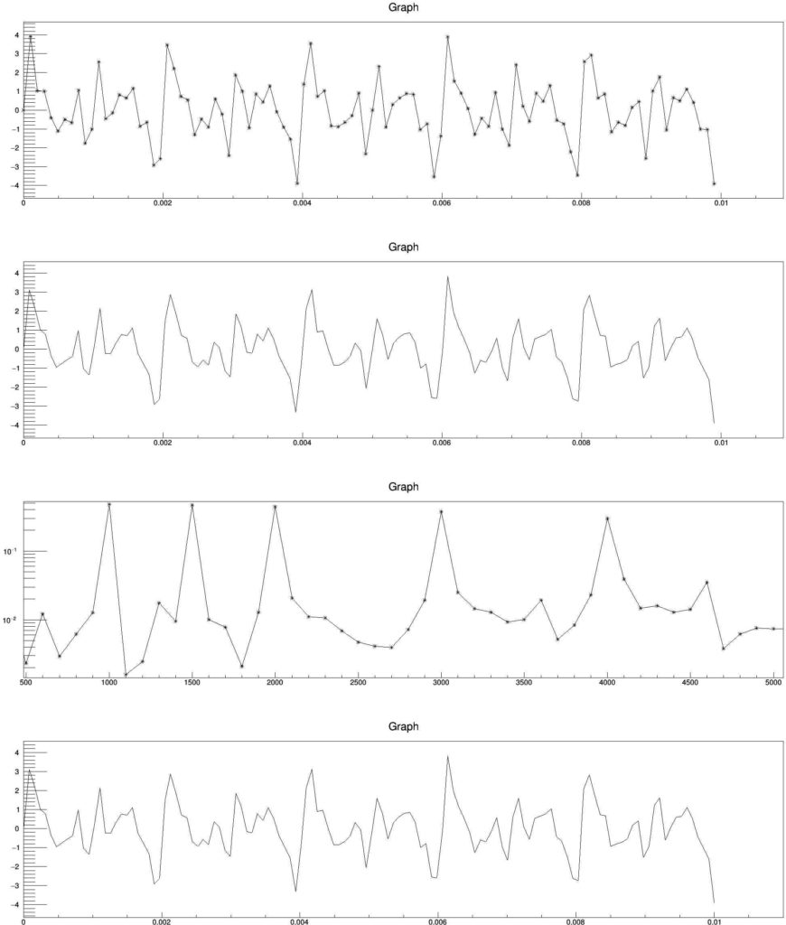
Now if you change only maxDataPt parameter
const Long64_t maxDataPt = pow(2,18);
Then the d-FFT plot will change to this.
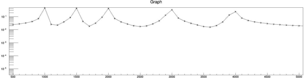
So, it is clearly visible that the quality of the d-FFT plot increased significantly by only increasing the data points, whereas, the original input data is same.
Now if the input data points is increased by changing maxGenPt
const Long64_t maxGenPt = 1000;
Then, the d-FFT plot will look like this.
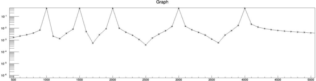
As, you can see here, by increasing the data points, the quality of the plot increased but the resolution remains the same. Now, we will change the tPD and see what happens.
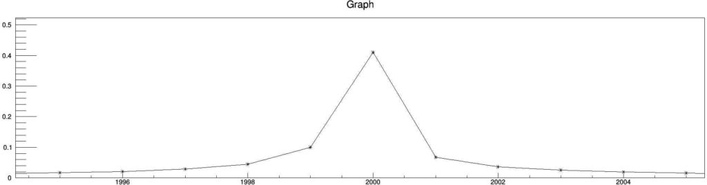
const double tPD = 1.;
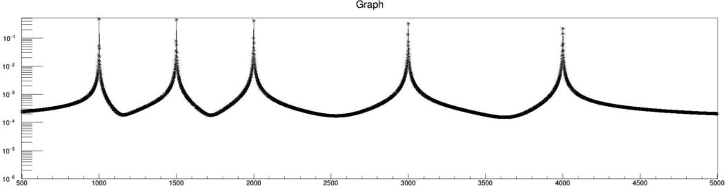
So, by increasing the tPD by $$100\times$$, we could increase the resolution by $$100\times$$. Here is the zoomed view of the $$2000\,\text{Hz}$$ peak. The resolution is $$1\,\text{Hz}$$.
Small Discussion
So, this is it guys. Go nuts with this code. Do some experiments. Add noise to each sine wave using gRandom->Gaus(xx,xx). Explore a little nit.
One more thing. I did not talk about the inverse d-FFT code here. It is pretty much simple and straight forward. But only thing to be reminded is that the input for this function has to be complex numbers. That is why I passed the output of the d-FFT directly without elimination the imaginary part.
Thank you for paying attention.
Enjoy